Circuit Tracing: An in-depth explanation about creating interpretability circuits
How do we extract interpretability circuits from transcoders?
Introduction
Large language models can often feel like inscrutable black boxes: they generate text with astonishing fluency, but the internal computations that drive their outputs remain hidden from us. Recently, I came across the paper “Transformers Find Interpretable LLM Feature Circuits”
The key idea is to treat a model as a computational graph of interacting components. By tracing attribution scores through this graph, we can identify the contributions of earlier-layer features and heads to later-layer representations, and eventually reconstruct causal circuits inside the model. Along the way, I discuss the theoretical foundation for this approach, show how feature vectors must be updated as we traverse the graph, and present algorithms for discovering important computational paths.
To make this more tangible, I finish with a case study on a small transformer trained on TinyStories, a dataset of fairytales. Here, interpretability techniques reveal exactly how the model encodes the familiar opening “Once upon a time”—uncovering the features and attention heads responsible for producing it.
What is a Transcoder?
Transcoders are a new way of peeking inside the black box of transformers. Traditionally, researches have used sparse autoencoders (SAEs)
Transcoder’s Architecture
At its core, a transcoder is a simple but powerful idea: we replace a transformer’s original MLP sublayer with a wider, sparse approximation that is (hopefully) easier to interpret. Concretely, a transcoder is just a one-hidden-layer ReLU MLP that learns to mimic the input-output behavior of the original MLP. Given an input activation vector $x \in \mathbb{R}^{d_{\text{model}}}$ the transcoder computes an intermediate sparse feature vector:
\[z_{\text{TC}}(x) = \text{ReLU}({W_{\text{enc}}}x) + b_{\text{enc}}\]where $W_{\text{enc}} \in \mathbb{R}^{d_\text{features} \times d_{\text{model}}}$ maps the input into a higher-dimensional “feature space” ($d_{\text{features}} \gg d_{\text{model}}$) and $b_{\text{enc}}$ is a bias term. Each component of $z_{\text{TC}}(x)$ represents the activation of a sparse feature.
The decoder stage then maps these features back into the model’s hidden space:
\[\text{TC}(x) = W_{\text{dec}}z_{\text{TC}}(x) + b_{\text{dec}},\]where $W_{\text{dec}} \in \mathbb{R}^{d_{\text{model}} \times {d_{\text{features}}}}$ and $b_{\text{dec}}$ reconstruct the MLP’s output. Intuitively, the encoder decides which features should fire, while the decoder decides how each feature contributes to the final output.
To train transcoders, we minimize a loss that balances faithfulness to the original MLP with sparsity of activations:
\[\mathcal{L}_{\text{TC}}(x) = \| \text{MLP}(x) - \text{TC}(x) \|_2^2 + \lambda_1 \| z_{\text{TC}}(x) \|_1\]where the first term ensures the transcoder closedly matches the true MLP outputs, and the second term (with hyperparameter $ \lambda_1 $) encourages sparse activations, making the features easier to interpret.
In short, transcoders trade a little extra width for a lot of interpretability: they give us a sparse, feature-level view of how information flows through MLP sublayers, without losing track of the original model’s computations.

Circuit tracing
With transcoders in hand, we can go a step further and actually trace the circuits that transformers use to solve tasks. The idea is simple: instead of asking how individual neurons connect, we ask how features discovered by transcoders in one layer connect to features in later layers. Suppose we found a feature in layer $\text{l’}$ that activates on certain tokens with a clear pattern (for example, semicolons after a year token
Computing the Attributions between Transcoder Feature Pairs
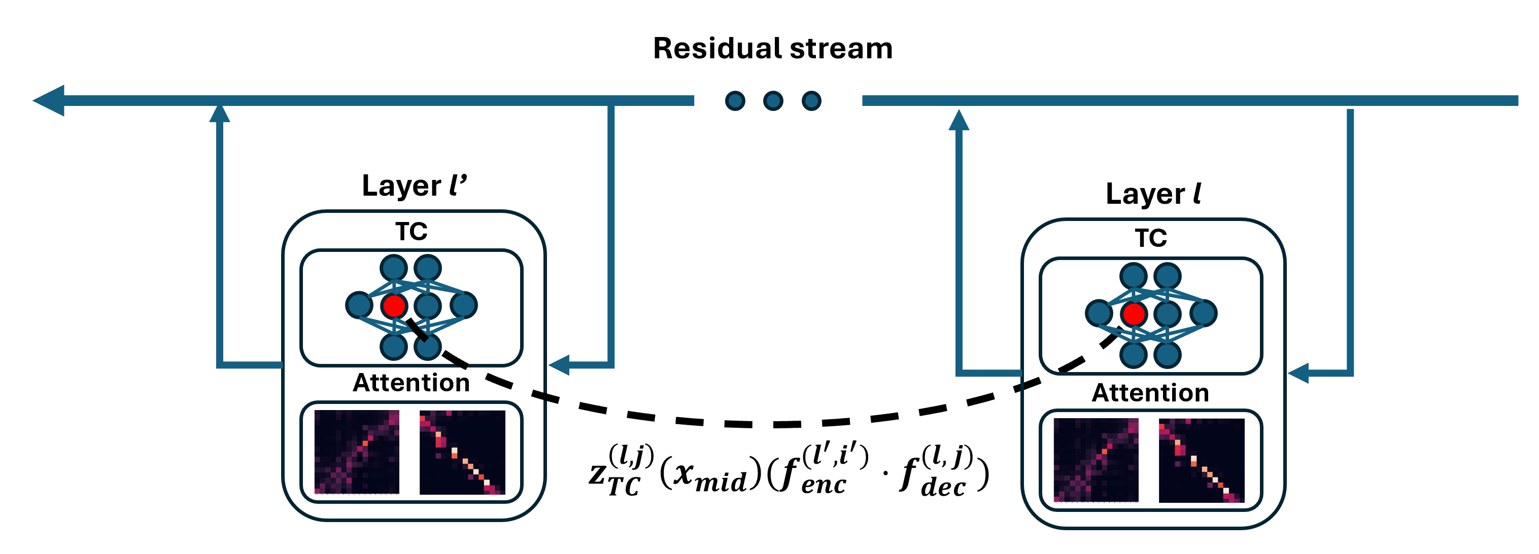
To understand how circuits are build, we start by giving a way of measuring the connection between two transcoder features. With transcoders, this turn out to be extremely simple. Formally, let $z^{(l,i)}_{\text{TC}}(x^{(l,t)}_{\text{mid}})$ denote the scalar activation of the $i$-th feature in the layer $l$ transcoder on token $t$, given the MLP input $x^{(l, t)}_{\text{mid}}$. Then for $l \lt l’$ the contribution of feature $ i $ in transcoder $ l $ to the activation of feature $ i’ $ in transcoder $ l’ $ is:
\[z^{(l,i)}_{\text{TC}}\left(x^{(l,t)}_{\text{mid}}\right) \cdot \left( f^{(l,i)}_{\text{dec}} \cdot f^{(l',i')}_{\text{enc}} \right) \tag{1}\]Here:
- $z^{(l,i)}_{\text{TC}}(x^{(l,t)}_{\text{mid}})$ is the activation of the earlier feature — this depends on the current input.
- $f^{(l,i)}_{\text{dec}}\cdot f^{(l’,i’)}_{\text{enc}}$ is the dot product between the earlier feature’s decoder vector and the later feature’s encoder vector — this is input-invariant once the transcoder is trained.
This clean factorization gives us the best of both worlds:
- An input-invariant term that tells us how features are generally connected across the model.
- An input-dependent term that tells us how much a feature mattered for the specific input at hand.
Now we’ll see how to derive equation 1. We are interested in the activation of feature $ i’ $ in transcoder layer $ l’ $ that activates on token $ t $. The activation is given by:
\[z_{\text{TC}}^{(l', i')}(x_{\text{mid}}^{(l', t)}) = \text{ReLU}(f_{\text{enc}}^{(l', i')} \cdot x_{\text{mid}}^{(l', t)} + b_{\text{enc}}^{(l', i')})\]where $f_{\text{enc}}^{(l’, i’)}$ is the $ i-th $ row of $W_{\text{enc}}$ for the layer $ l’ $ transcoder and $b_{\text{enc}}^{(l’, i’)}$ is the learned encoder bias for feature $ i’ $ in the layer $ l’ $ transcoder. Now, we know that this feature is active (i.e. $z_{\text{TC}}^{(l’, i’)}(x_{\text{mid}}^{(l’, t)}) \gt 0$) and it’s reasonable to assume that this firing is not given by the bias term. We can therefore ignore $b_{\text{enc}}^{(l’, i’)}$. Then, since $z_{\text{TC}}^{(l’, i’)}(x_{\text{mid}}^{(l’, t)}) \gt 0$ we can further ignore the $ \text{ReLU} $, leaving us only with:
\[z_{\text{TC}}^{(l', i')}(x_{\text{mid}}^{(l', t)}) \approx f_{\text{enc}}^{(l', i')} \cdot x_{\text{mid}}^{(l', t)}\]Thanks to the residual connections in transformers $x_{\text{mid}}^{(l’, t)}$ can be decomposed as the sum of the outputs of all previous components in the model (MLPs and Attention blocks). For instance, in a two-layer model, if $x_{\text{mid}}^{(2, t)}$ is the input for the second MLP sublayer:
\[x_{\text{mid}}^{(2, t)} = \sum_{h}\text{attn}^{(2, h)}(x_{\text{pre}}^{(2, t)};x_{\text{pre}}^{(2, 1:t)}) + \text{MLP}(x_{\text{mid}}^{(1, t)}) + \sum_{h}\text{attn}^{(1, h)}(x_{\text{pre}}^{(1, t)};x_{\text{pre}}^{(1, 1:t)})\]Now, assume that we want to consider how much a feature from the first MLP layer contributes to a feature in the second layer. Because of linearity, the amount of $\text{MLP}^{(1)}(x_{\text{mid}}^{(1, t)})$ that contributes to $f_{\text{enc}}^{(2, i’)} \cdot x_{\text{mid}}^{(2, t)}$ is given by:
\[f_{\text{enc}}^{(2, i')} \cdot \text{MLP}^{(1)}(x_{\text{mid}}^{(1, t)}) \tag{2}\]This is generalizable for understanding the contribution of $ \text{MLP} \ l $ to the activation of feature $ i’ $ in transcoder $ l’ $, with $ l \lt l’ $. Now, we can start from here to find the attribution of feature $ i $ in transcoder $ l $ with respect to feature $ i’ $ in transcoder $ l’ $.
In particular, we know that transcoders are trained to reconstruct MLP outputs. So, if layer $ l $ transcoder is a good approximation to the layer $ l $ MLP, then $\text{MLP}^{(1)}(x_{\text{mid}}^{(l, t)}) \approx \text{TC}^{(l)}(x_{\text{mid}}^{(l, t)})$. Hence, we can use this approximation in Equation 2 to obtain:
\[f_{\text{enc}}^{(l', i')} \cdot \text{MLP}^{(l)}(x_{\text{mid}}^{(l, t)}) \approx f_{\text{enc}}^{(l', i')} \cdot \text{TC}^{(l)}(x_{\text{mid}}^{(l, t)}) \tag{3}\]Equation 3 tells us the whole contribution of $\text{TC}^{(l)}$ on feature $ i’ $ in transcoder $ l’ $. To extract individual feature attributions, we can leverage transcoder’s linearity $\text{TC}^{(l)}(x_{\text{mid}}^{(l, t)}) = \sum_{\text{feature} \ j} z_{\text{TC}}^{(l, j)}(x_{\text{mid}}^{(l, t)})f_{\text{dec}}^{(l, j)}$. This is how we can decompose the transcoder attribution into its features contributions to feature $ i’ $ in transcoder $ l’ $.
Thus, we have:
\[f_{\text{enc}}^{(l', i')} \cdot \text{MLP}^{(l)}(x_{\text{mid}}^{(l, t)}) \approx f_{\text{enc}}^{(l', i')} \cdot \sum_{\text{feature} \ j} z_{\text{TC}}^{(l, j)}(x_{\text{mid}}^{(l, t)})f_{\text{dec}}^{(l, j)} \tag{4}\]Therefore, the attribution of feature $ i $ in layer $ l $ with respect to feature $ i’ $ in transcoder $ l’ $ is given by:
\[z_{\text{TC}}^{(l, j)}(x_{\text{mid}}^{(l, t)})(f_{\text{enc}}^{(l', i')} \cdot f_{\text{dec}}^{(l, j)}) \tag{5}\]where we have just put $f_{\text{enc}}^{(l’, i’)}$ inside the parenthesis since $z_{\text{TC}}^{(l, j)}(x_{\text{mid}}^{(l, t)})$ is a scalar.

Computing the Attributions through Attention Heads
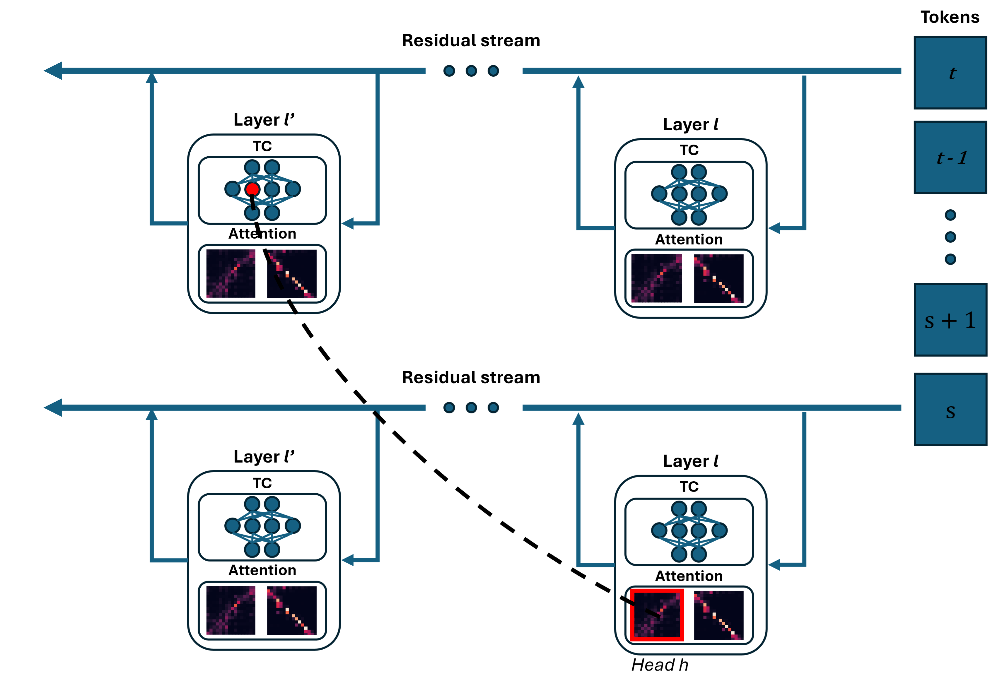
So far, we have focused on tracing how a lower-layer transcoder feature directly contributes to a higher-layer transcoder feature at the same token position. However, transcoder features can also be mediated by attention heads, which requires us to extend the analysis. Attention can be decomposed into two circuits, a QK (query-key) circuit, which decides where to move information from and to, and the OV (output-value) circuit, which decides what information to move
This can be decomposed into a sum over source tokens $s$:
\[f^{(l',i')}_{\text{enc}} \cdot \sum_{\text{source token}\,s}\text{score}^{(l,h)}\big(x^{(l,t)}_{\text{pre}}, x^{(l,s)}_{\text{pre}}\big) \, W^{(l,h)}_{\text{OV}}\,x^{(l,s)}_{\text{pre}} \tag{7}\] \[=\sum_{\text{source token}\,s}\text{score}^{(l,h)}\big(x^{(l,t)}_{\text{pre}}, x^{(l,s)}_{\text{pre}}\big) \, \big(f^{(l',i')}_{\text{enc}}\big)^{T}W^{(l,h)}_{\text{OV}}\,x^{(l,s)}_{\text{pre}} \tag{8}\] \[=\sum_{\text{source token}\,s}\text{score}^{(l,h)}\big(x^{(l,t)}_{\text{pre}}, x^{(l,s)}_{\text{pre}}\big) \, \big(\big(W^{(l,h)}_{\text{OV}}\big)^{T}f^{(l',i')}_{\text{enc}}\big) \cdot x^{(l,s)}_{\text{pre}} \tag{9}\]where from (7) to (8) we put $f^{(l’,i’)}_{\text{enc}}$ inside the parenthesis since $\text{score}^{(l,h)}\big(x^{(l,t)}_{\text{pre}}, x^{(l,s)}_{\text{pre}}\big)$ are scalars for all $s$ and from (8) to (9) we used $A\cdot B = (B^{T}\cdot A^{T})^{T}$.
Thus, the contribution of source token $s$ at layer $l$ through head $h$ can be written as:
\[\text{score}^{(l,h)}\big(x^{(l,t)}_{\text{pre}}, x^{(l,s)}_{\text{pre}}\big) \, \big(\big(W^{(l,h)}_{\text{OV}}\big)^\top f^{(l',i')}_{\text{enc}}\big) \cdot x^{(l,s)}_{\text{pre}} \tag{10}\]So now, for a given feature $i’$ that fires in layer $l’$ on token $t$, we can now trace back all its influences. We can calculate the contribution from every previous-layer feature (Equation 5) and from any source token $s$, with $s \lt t$, processed from attention head $h$ (Equation 10).
The final step is to note that $x^{(l,s)}_{\text{pre}}$ itself can be decomposed again into the output of MLP sublayers and attention heads, allowing us to recurse back until the token embeddings. To visualize this better, assume that you know that on layer 8 feature 2020 is firing on token 5. You apply Equation (5) and you find that most of the contribution is coming from feature 1546 in layer 4, activating on token 5. Your next question is: why is feature 1546 activating? So, given equations 5 and 10, you can recurse back, constructing a computational graph, until you get to the first layer of your model, in which you can see the tokens that make your feature fire. In the next subsection, I’ll explain how to get the attribution graph.

Tracing Features Back
So far, we’ve seen how to calculate the attribution from an earlier-layer transcoder feature or attention head to a later-layer feature. But that’s only half of the story. To truly understand the model’s behavior, we need to flip the perspective: what contributes to these earlier-layer features or heads in the first place?
This bring us to the idea of recursive attribution tracing, that can be expressed as follows:
Starting from the final feature vector we care about (e.g. $f_{enc}^{(l’, i’)}$ for $i$-th feature in layer $l’$) we move backwards step by step. At each node - earlier transcoder feature or attention head - we compute how much that node contributes to the current feature vector using Equations 5 and 10. We than update our feature vector accordingly and continue tracing backwards until we reach the inputs.
Now, why do we need to update the feature vector step? Recall that we are calculating attributions for a particular feature in a given layer computing the inner product beween its feature vector and its inputs $f_{\text{enc}}^{(l’, i’)} \cdot x_{\text{mid}}^{(l, t)}$. So the feature vector represents the lens thruogh with we measure attribution, and that lens changes as activations are transformed along the computational path
So our new feature feature vector will be $f=f’\cdot A$. This way, $f$ is aligned with the input space and the attribution remains valid one step earlier in the graph. The same principles applies for MLP and Attention nodes that we have in the graph: the feature vector must be updated to remain consistent with the representation space of the preceding layer.
So, in order to compute the new feature vector $f$ through node $c$ starting from $f’$ we’ll use the following contraint given from Equation 11:
\[a' = f' \cdot y = f \cdot x\]When node $c$ is an attention head in layer $l$, we have $y = x_{\text{mid}}^{(l, t)}$, so:
\[a' = f' \cdot y = f' \cdot x_{\text{mid}^{(l, t)}} = f' \cdot \sum_{h}\sum_{s}\text{score}^{(l,h)}\big(x^{(l,t)}_{\text{pre}}, x^{(l,s)}_{\text{pre}}\big) \, W^{(l,h)}_{\text{OV}}\,x^{(l,s)}_{\text{pre}}\]However, assume that we are tracing the attribution through head $h$ of a source token at position $s$. Therefore, we have $x = x_{\text{pre}}^{(l, s)}$ and the updated feature vector will be:
\[a' = f' \cdot \text{score}^{(l,h)}\big(x^{(l,t)}_{\text{pre}}, x^{(l,s)}_{\text{pre}}\big) \, W^{(l,h)}_{\text{OV}}\,x^{(l,s)}_{\text{pre}}\] \[= f' \cdot \text{score}^{(l,h)}\big(x^{(l,t)}_{\text{pre}}, x^{(l,s)}_{\text{pre}}\big) \, W^{(l,h)}_{\text{OV}}\,x\] \[= \big(f' \cdot \text{score}^{(l,h)}\big(x^{(l,t)}_{\text{pre}}, x^{(l,s)}_{\text{pre}}\big) \, W^{(l,h)}_{\text{OV}}\big)\,x\] \[= f \cdot x\]Hence:
\[f = f' \cdot \text{score}^{(l,h)}\big(x^{(l,t)}_{\text{pre}}, x^{(l,s)}_{\text{pre}}\big) \, W^{(l,h)}_{\text{OV}} \tag{12}\]In contrast, if $c$ is a transcoder feature then $y = x_{\text{post}}^{(l, t)}$, so we have:
\[a' = f' \cdot x_{\text{post}}^{(l, t)} = f' \cdot \text{MLP}^{(l)}(x_{\text{mid}}^{(l, t)}) \approx f' \cdot \text{TC}^{(l)}(x_{\text{mid}}^{(l, t)})\] \[= f' \cdot \sum_{j}z_{\text{TC}}^{(l, j)}(x_{\text{mid}}^{(l, t)}) \cdot f_{\text{dec}}^{(l, j)}\]Moreover, from the definition of transcoder, we have that $z_{\text{TC}}^{(l, t)}(x_{\text{mid}}^{(l, t)}) = f_{\text{enc}}^{(l, j)} \cdot (x_{\text{mid}}^{(l, t)})$. Therefore, we obtain:
\[a' = f' \cdot x_{\text{post}}^{(l, t)} = f' \cdot \sum_{j} f_{\text{enc}}^{(l, j)} \cdot (x_{\text{mid}}^{(l, t)}) \cdot f_{\text{dec}}^{(l, j)}\]From this, we can just insert inside the sum $f’$ thanks to the linearity of the inner product:
\[a' = f' \cdot x_{\text{post}}^{(l, t)} = f' \cdot \sum_{j} f_{\text{enc}}^{(l, j)} \cdot (x_{\text{mid}}^{(l, t)}) \cdot f_{\text{dec}}^{(l, j)}\] \[=\sum_{j} \big(f_{\text{enc}}^{(l, j)} \cdot (x_{\text{mid}}^{(l, t)})\big) \cdot \big( f' \cdot f_{\text{dec}}^{(l, j)}\big)\]And from this, knowing that our $x = (x_{\text{mid}}^{(l, t)})$ and assuming we are interested in the contribution of feature $j$ from layer $l$ it’s easy to see that:
\[f = \big( f' \cdot f_{\text{dec}}^{(l, j)}\big) \cdot f_{\text{enc}}^{(l, j)} \tag{13}\]There is, however, an important caveat. Transformer architectures insert a LayerNorm operation before every MLP and attention sublayer. This nonlinearity complicates attribution because it rescales and recenters activations. Fortunately, prior work provides intuition and justification for approximating LayerNorm as a linear scaling transformation. Neel Nanda here argues that it behaves roughly like multiplying the input by a constant, and Dunefsky & Cohan
At this point, we’re able to trace back our feature vector in any block of our transformer model. In other words, we’re ready to construct the attribution graph!
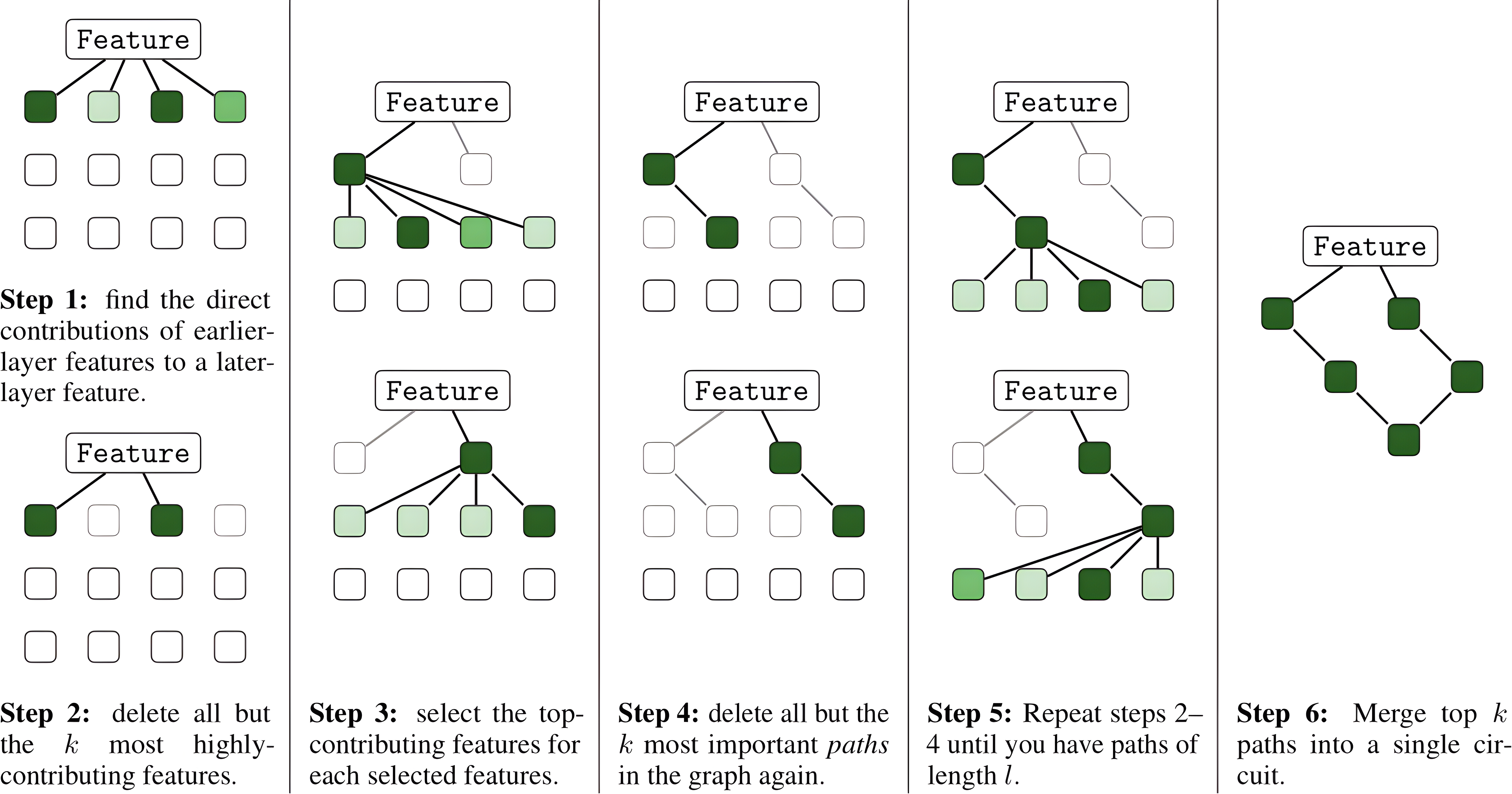
Computing the Attribution Graph
The full circuit-finding algorithm is basically a way of “tracing back the breadcrumbs” to figure out which parts of a transformer are truly responsible for a feature lighting up. Imagine you notice a neuron firing strongly in a late layer — the algorithm asks: what earlier features, attention heads, or even embeddings made this happen? To answer that, it builds computational paths step by step, moving backwards through the network. At each step, it looks at all possible contributors, scores them by how much they mattered, and then keeps only the top few. This greedy approach means we don’t get lost in the exponential explosion of possible paths, but we still hang onto the most important ones. After running this process for several steps, you end up with a collection of “candidate stories” — paths that explain how the signal was built. But paths alone can be messy: the same node might appear in several different explanations, and if we just add everything up we’d double-count. That’s why the second stage of the algorithm takes all those paths and merges them into a single graph. In this graph, every node and every edge gets an attribution score that represents its total contribution across all explanations. And just to stay honest, we also allow for “error nodes” — placeholders that capture the fact that we didn’t include every possible path or that our approximations (like treating LayerNorm as linear) aren’t perfect. The end result is a clear, interpretable circuit diagram showing how the model built up the feature of interest.

An example using fairytales
To make things more concrete, let’s look at an example drawn from a model I recently trained on TinyStories, a dataset of short fairytales (you can find it here). One of the most characteristic phrases in this dataset is the classic opening “Once upon a time”. The model reproduces this phrase frequently, and I was curious to see where in the network this pattern is “stored” and how it emerges.
To start, I probed the activations inside the model when it processed this phrase. Looking specifically at the token “a” in “Once upon a time”, I found that feature 1932 in layer 1 showed particularly strong activation.
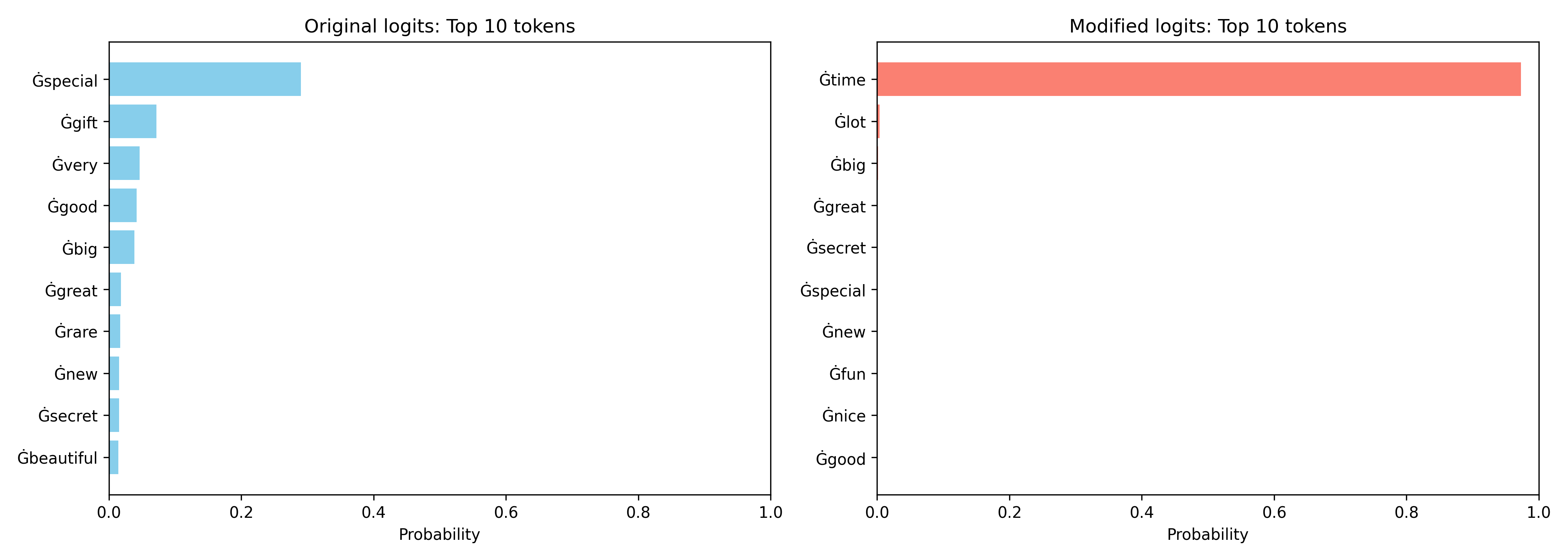
Interestingly, whenever this feature lights up, the model becomes strongly biased towards predicting the token “time” as the next word. This suggests that feature 1932 has learned to specialize in carrying forward the “Once upon a … time” motif.
To validate this hypothesis, I ran an intervention: I manually activated feature 1932 in contexts where it would not normally fire. Here, no matter the surrounding text, the model tried to output “time” immediately afterward.

This confirms that the feature does not simply correlate with the training distribution, but actually plays a causal role in driving the model toward producing this phrase.
Going deeper, I also used the circuit-finding method described earlier to trace which components contribute to the activation of feature 1932. Two particularly clear computational paths emerged:
- Path 1:
mlp1@2@2 ← mlp0tc[2915]@2: 2.8 ← attn0[3]@0: 0.24 - Path 2:
mlp1@2@2 ← mlp0tc[2915]@2: 2.8 ← attn0[2]@1: 0.21
This notation means that feature 1932 in layer 1 is being modulated by feature 2915 in layer 0, which itself receives contributions from attention head 3 at token position 0 and attention head 2 at token position 1. In plain language: the feature that predicts “time” is activated through a chain that depends on the tokens “once” and “upon”.
Altogether, this paints a coherent picture. The model has carved out a small, interpretable circuit that detects the prefix “once upon a …” and channels this information forward to bias the output toward “time”. In other words, the phrase “Once upon a time” has been distilled into a mechanistic substructure inside the model.
This example highlights the promise of feature- and circuit-level interpretability: even in a small two-layer transformer, we can begin to see how specific linguistic motifs are encoded, propagated, and ultimately expressed in the model’s predictions.
Conclusions
By following attributions backward through the network and systematically building computational paths into circuits, we gain a concrete picture of how language models organize knowledge internally. What initially appears as an opaque “black box” turns into a structured system of features, heads, and layers that cooperate to produce meaningful outputs.
The case study on “Once upon a time” illustrates this beautifully: a specific feature in layer 1, modulated by lower-layer components attending to “once” and “upon”, reliably pushes the model to predict “time”. This shows that the model has not just memorized text, but carved out specialized circuits to handle recurring linguistic motifs.
Of course, this is just one small example in a tiny model. The ultimate challenge is to scale these methods to much larger architectures and more abstract concepts, where the circuits will be deeper and more intertwined. Still, even in this setting, we see a glimpse of what is possible: by peeling back the layers of the network, we can begin to map out the hidden structures that give rise to language understanding.
Enjoy Reading This Article?
Here are some more articles you might like to read next: