Your Favourite Genomic Model knows more than you think

Introduction

In the world of Natural Language Processing, we often draw a sharp line between discriminative models like BERT (designed to understand and classify) and generative models like GPT (designed to create).

But what if this boundary is more subtle than you think? What if your favourite BERT-style genomic model could surprise you by generating coherent text just after one hour of finetuning?

In this post, we’ll explore how the MLM objective can be mathematically reframed as a Discrete Diffusion process, effectively turning a “static” classifier into a powerful generator. I wanted to test this theory using DNABERT-2 to generate synthetic human enhancers and validate them against real ones. All of the code can be found here.

Masked Language Modeling (MLM)

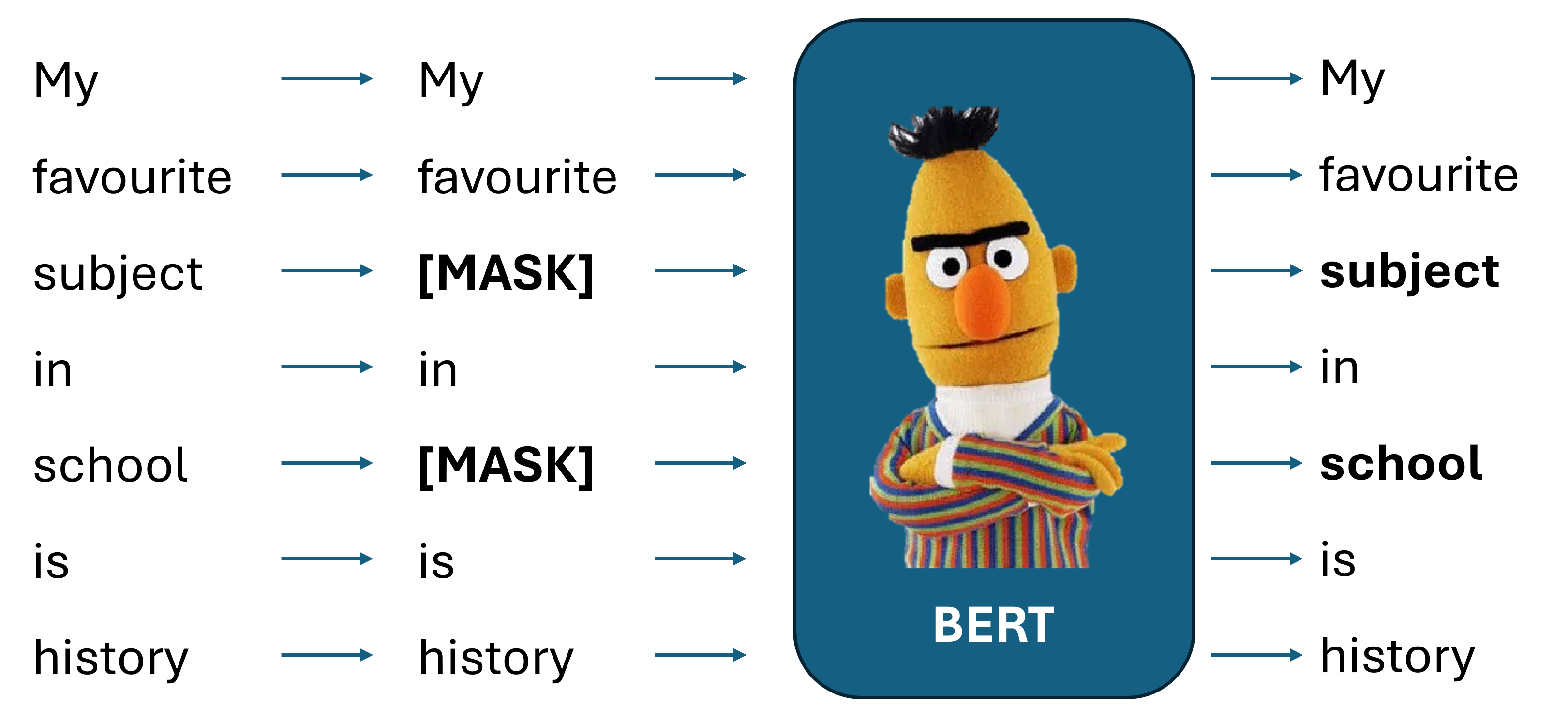
Masked Language Modeling (MLM) is essentially a sophisticated, high-speed game of “fill-in-the-blanks” designed to teach AI models deep contextual understanding. Unlike traditional models that read text sequentially from left to right—predicting the next word based only on what came before—BERT uses MLM to become truly bidirectional. It takes a complete sentence and hides 15% of the words, but it does so using a clever 80/10/10 strategy to prevent the model from becoming lazy.

Specifically, for that 15% of chosen words:

• 80% are replaced with a [MASK] token (forcing the model to rely on context).
• 10% are replaced with a random word (forcing the model to act as a “spell checker” that detects logic errors).
• 10% are left unchanged (ensuring the model still values the actual word when it is present).

By forcing the model to analyze these surrounding “clues” from both directions, MLM enables BERT to develop a much richer grasp of language nuances, syntax, and semantics. This is why BERT can easily distinguish between “bank” (a river) and “bank” (a financial institution) based entirely on the words sitting next to it.

Discrete Diffusion

Diffusion models are a class of latent variable models that are originally designed for continuous domains. A diffusion model is consisting of a forward diffusion process. Given a sample \(x_{0} \sim q(x_{0})\), a Markov chain of latent variables \(x_{1}, ..., x_{T}\) are produced in the forward process by progressively adding a small amount of Gaussian noise to the sample:

\begin{equation} q\left(x_{t} \mid x_{t-1} \right) = \mathcal{N}(x_{t};\sqrt{1 - \beta_{t}}x_{t-1}, \beta_{t}\mathbb{I}) \end{equation}

where \(\beta_{t} \in \left(0, 1\right)\) is a noise schedule controlling the step size of adding noise (i.e. the [MASK] token).

It can be shown that if \(\beta_{t}\) is small enaugh, the reverse process \(q\left(x_{t-1} \mid x_{t} \right)\) is also a Gaussian, learned by the parametrized model.

\begin{equation} p_{\theta}\left(x_{t-1} \mid x_{t}, t\right) = \mathcal{N}\left(x_{t-1};\mu_{\theta}\left(x_{t}, t\right), \Sigma_{\theta}\left(x_{t}, t\right)\right) \end{equation}

where \(\mu_{\theta}\) and \(\Sigma_{\theta}\) can be implemented using a U-Net or a Neural Network. When conditioning also on \(x_{0}, p_{\theta}\left(x_{t-1} \mid x_{t}, x_{0}\right)\) has a closed form so we can use Kulback-Leider divergence as a loss for our model.

For discrete domains, each element of \(x_{t}\) is a discrete random variable with K categories. Denote \(x_{t}\) as a stack of one-hot vectors, the process of adding noise can be written as:

\begin{equation} q_{\left(x_{t} \mid x_{t-1}\right)} = \text{Cat}\left(x_{t}; p = x_{t-1} Q_{t}\right) \end{equation}

where \(\text{Cat}(z)\) is a categorical distribution (i.e. the random variable can take one of K possible categories) and \(Q_{t}\) is a transition matrix that is applied to each token in the sequence independently.

Therefore, for a given token, using Bayes theorem, it is easy to obtain that:

\begin{equation} q\left(x_{t-1} \mid x_{t}, x_{0}\right) = \text{Cat} \big( x_{t-1}; p = \frac{x_{t} Q^{T}_{t} \odot x_{0}\bar{Q}_{t-1}}{x_{0}\bar{Q}_{t}x_{t}^{T}} \big) \end{equation}

where \(\bar{Q}_{t} = Q_{1}Q_{2} \dots Q_{t}\). So with \(q\left(x_{t-1} \mid x_{t}, x_{0}\right)\) we can learn to reverse the diffusion process.

BERT is a one-step diffusion model

Luckily for us, it can be shown that the Loss for a Discrete Diffusion model can be transformed into an MLM loss under the following conditions:

1. Zero-Masking Probabilities: a clear input (i.e. an input token which is non-masked) is never masked.
2. Carry-Over Unmasking: an unmasked token remains unchanged during reverse diffusion.

If so, the loss function can be rewritten as:

But this is exactly the MLM loss function. So, a BERT-based model can be finetuned to be used as a diffusion model. At each step we replace a different proportion $p$ of tokens with [MASK] using a variable $p \in (0.10, 0.90)$. In this way, the model is trained to replace [MASK] tokens with real ones in different conditions. During generation, we start from a completely masked sequence, and, at each denoising step, BERT will replace some proportion [MASK] with generated tokens, until the full sequence is constructed.

DNABERT generates enhancers

Now that we know that we can finetune BERT to produce sequences, let’s try it with DNABERT. DNABERT is a BERT-based genomic model trained on a huge collection of DNA sequences. It has archieved state-of-the-art results in many genomic tasks, including enhancer prediction, promoter identification, and splice site prediction.

To make a choice, I decided to finetune DNABERT-2 with enhancer sequences taken from the Genomic Understanding Evaluation (GUE) benchmark, available on HF here. In particular, I selected enhancers coming from the K562 cell line, and divided them into training and test sets.

The finetuning procedure follows what written in the preceeding paragraph, i.e. randomly masking a proportion $p$ of tokens from each sequence, with $p$ ranging from $0.10$ to $0.90$.

def collate_fn(self, batch, debug: bool = False) -> dict[str, torch.Tensor]:
        
        # Tokenize the sequences
        [...]

        # Extract ids and attention mask
        batch_input_ids = tok_out["input_ids"]
        batch_attention = tok_out["attention_mask"]

        # Get input shape
        B, L = batch_input_ids.shape

        # Clone input ids for the labels
        labels = batch_input_ids.clone()

        # Sample t ~ Uniform[0, 1)
        t = torch.empty(B, 1).uniform_(0.10, 0.90)
        alpha_t = self.alpha(t)
        p = 1 - alpha_t

        # Determine which tokens can be masked
        mask_candidate = (batch_attention == 1) & (~is_special)

        # Randomly select tokens to mask based on p
        rand = torch.rand_like(batch_input_ids, dtype=torch.float)
        mask_positions = (rand < p) & mask_candidate

        # Apply masking
        batch_input_ids[mask_positions] = self.tokenizer.mask_token_id

        # Set unmasked positions to -100 in labels (ignored by loss)
        labels[~mask_positions] = -100

        return {
            "input_ids": batch_input_ids,
            "attention_mask": batch_attention,
            "MLM_labels": labels,
            "t": t # to keep track of timesteps
        } 

This ensures that the model is able to reconstruct the input sequence for different masking proportions.

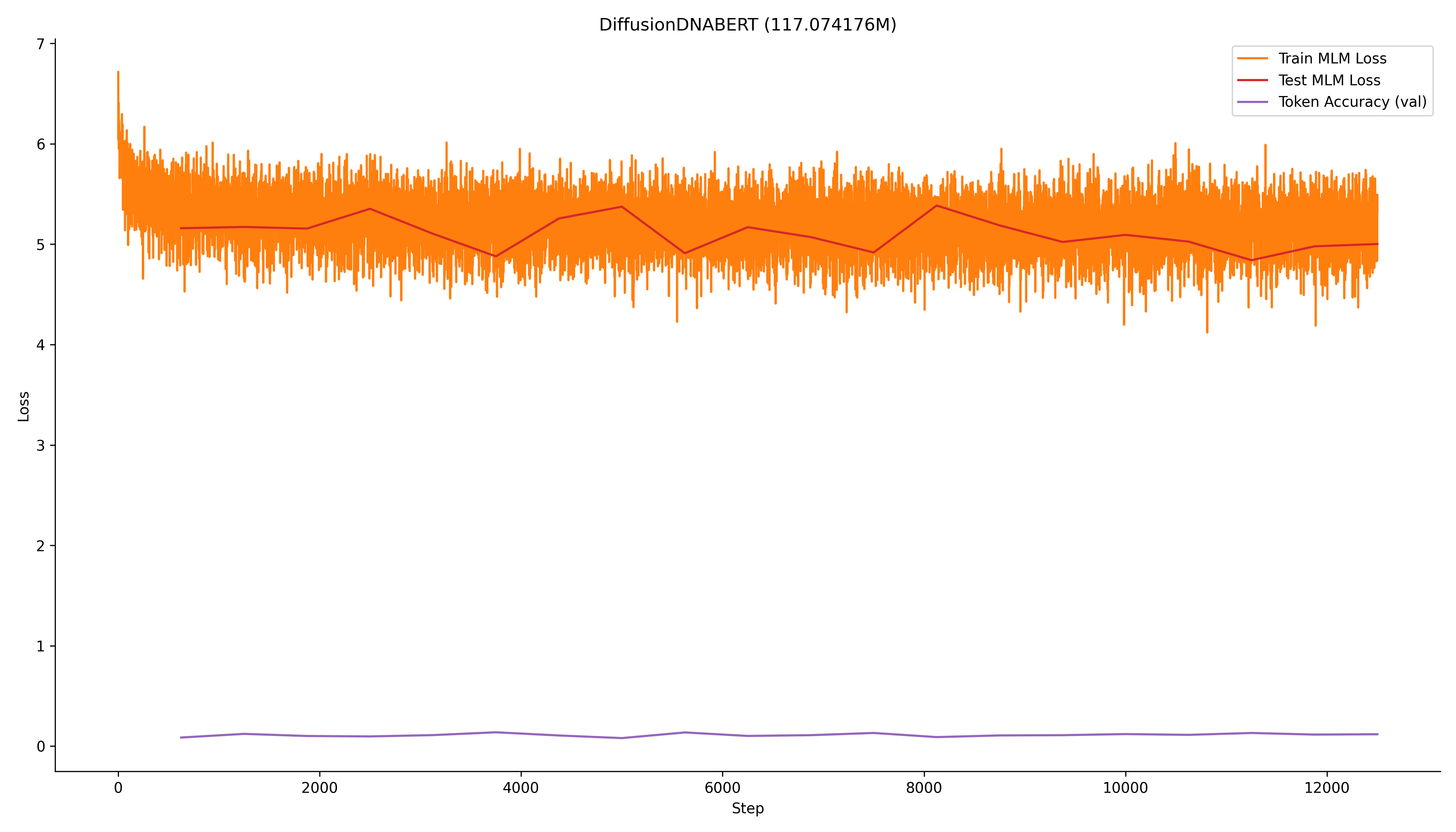
The model was finetuned for 20 epochs, maybe a little too much (but took less than an hour on my 4060 GPU), and the results are shown below.

Now that we have the model, let’s start generating something and see how good are the generated enhancer. But, first of all, how can I decide whether an enhancer is good or bad? And, most importantly, what is an enhancer? Following Barral et al., 2023:

Enhancers are cis-regulatory elements that can stimulate gene expression from distance, and drive precise spatiotemporal gene expression profiles during development. Functional enhancers display specific features including an open chromatin conformation, Histone H3 lysine 27 acetylation, Histone H3 lysine 4 mono-methylation enrichment, and enhancer RNAs production. [[…]] Their DNA sequences are composed of tissue-specific transcription factor (TFs) binding sites, conferring tissue specific activity.

So, an enhancer is a specific sequence that:

1. Usually is in an open-chromatin region so it must display some transcription factor binding sites.
2. Displays specific features like Histone H3 lysine 27 acetylation (H3K27ac) and Histone H3 lysine 4 mono-methylation (H3K3me1)

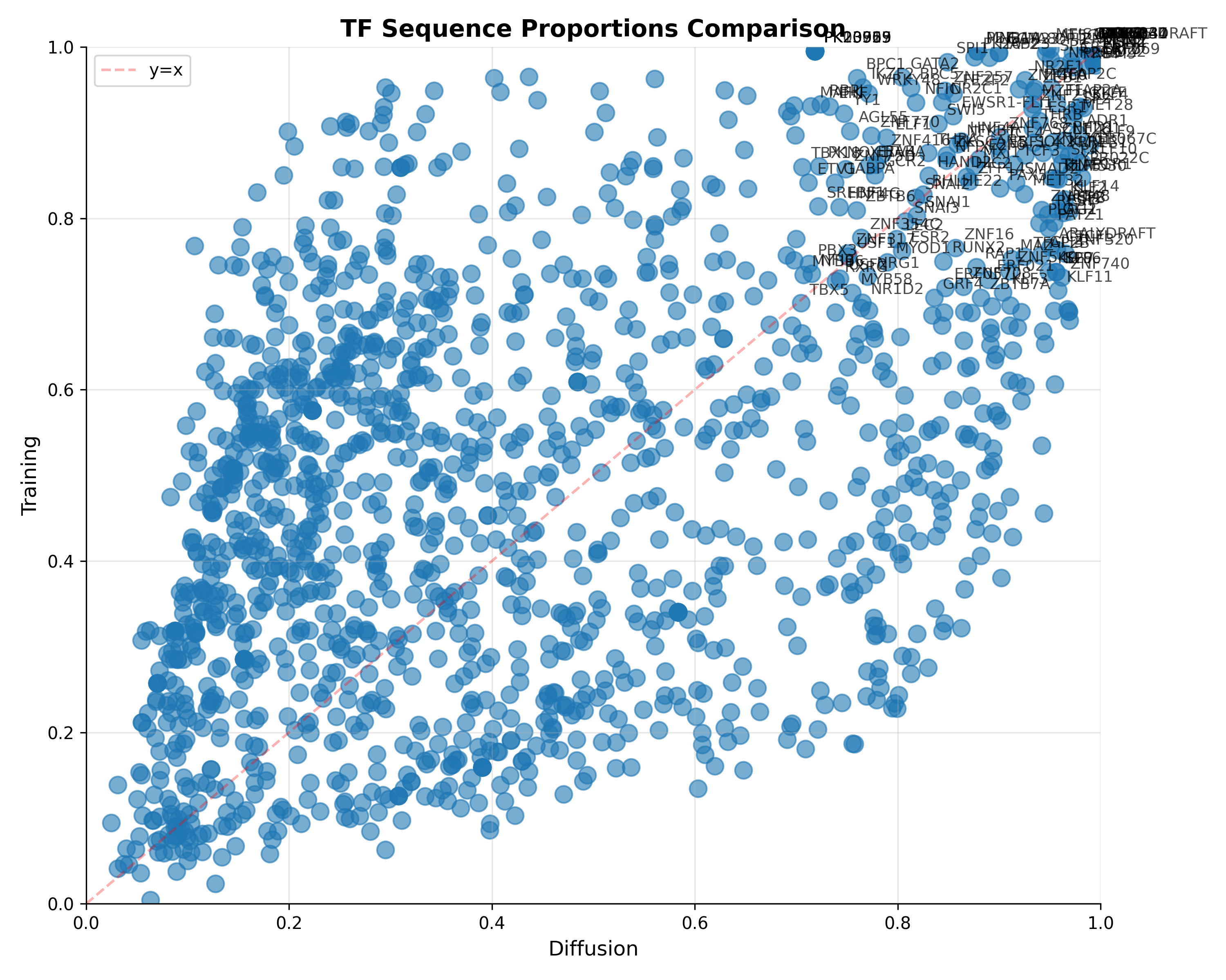
So let’s search for TFs and H3K27ac and H3K3me1 traits in our generated sequences. The TFs can be found screening different position frequency matrices (PFMs) against the generated and test sequences to see whether they share the same composition of TFs, while the Histone traits can be found using a DL model like Enformer. For the PFMs, I downloaded the human (redundant) collection from JASPAR.

Unfortunately, the H3K27ac head for K562 cells is not available in Enformer, but we can still measure the H3K3me1 trait. For this experiment, since Enformer context window is roughly 200kbp, I inserted my generated sequences (roughly 3000bp) into 200kbp random sequences, and measured the H3K3me1 trait. Below you can see an example:

So, I decided to create a bunch of 2000 sequences (as many as they are in the test set), measure their activity, to compare with the test set’s activity. In the end, the generated sequences seems to follow the same activity pattern, underlying a good generation.

Conclusions

This results seems promising, since in just one hour we passed from having an encoder to have a generative model which generates good human enhancers. So, for synthetic DNA generation, this suggests that instead of starting from scratch, we can take the massive genomic “knowledge” already stored in pre-trained models like DNABERT and “steer” it toward designing synthetic regulatory elements with specific functional goals.

However, for now the model is only capable of generating one type of sequences. I’m wondering whether working on the [CLS] token during generation could steer the model into producing more specific synthetic sequences (i.e. generating promoters or enhancers).

Ultimately, this experiment proves that these models are not just static lookup tables for genomic features. When we change our perspective on how to use them, we realize that your favourite genomic model knows more than you think.